
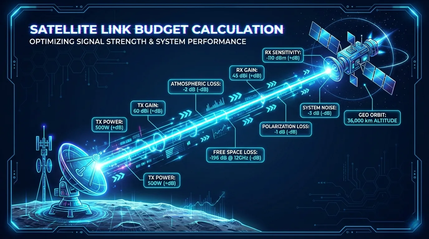
Satellite Link Budget Calculation with Example
Calculate a satellite link budget step by step: EIRP, antenna gain, FSPL, G/T, C/N0, C/N, uplink/downlink combination, rain loss, and link margin.
What changed: Replaced generic margin ranges with a reproducible 12 GHz GEO downlink example, corrected C/N0 and combined-link notation, added units and boundary conditions, and tied propagation and MODCOD claims to current ITU-R and ETSI documents.
A satellite link budget answers one practical question: after every gain and loss, does the received carrier exceed the modem's required threshold with enough margin for the target operating condition? A useful budget must name the direction, site, frequency, slant range, bandwidth or symbol rate, weather condition, availability target, equipment state, and threshold reference. Without those inputs, a margin number is not reproducible.
The core clear-sky downlink calculation is:
C/N0 = EIRP + G/T - FSPL - Lother + 228.6       dB-Hz
C/N  = C/N0 - 10 log10(Bn)                     dB
margin = available C/N - required C/N - implementation loss
All gains and losses above are logarithmic quantities. B_n is the receiver noise bandwidth in hertz, and 228.6 dB is the rounded logarithmic form of -10 log10(k) for Boltzmann's constant. The BIPM SI definition fixes k at exactly 1.380649 × 10⁻²³ J/K.
This guide develops the equations, then closes a complete numerical example. The example is an educational model with declared assumptions, not an operator design or equipment recommendation.
EIRP Explained | G/T Explained | C/N, C/N0, and Eb/N0
Inputs Required Before You Calculate
Create separate input sheets for the uplink and downlink. At minimum, record:
| Input group | Required values | Source of truth |
|---|---|---|
| Geometry | Earth-station coordinates, satellite longitude or ephemeris, elevation angle, slant range | Pointing calculation or operator data |
| Carrier | Uplink/downlink frequency, symbol rate, roll-off, occupied and noise bandwidth | Carrier plan and modem configuration |
| Transmit chain | Power at reference plane, feeder/filter losses, transmit antenna gain, pointing loss, backoff | Equipment data and measured commissioning values |
| Space segment | Per-carrier EIRP or G/T at the site, transponder gain/loading, IBO/OBO, beam contour | Operator link data, not beam-peak marketing values |
| Receive chain | Receive gain, feed loss, antenna temperature, receiver noise temperature, system noise temperature | Antenna/LNB data and noise-temperature calculation |
| Propagation | Gaseous, cloud, rain, scintillation, polarization and other path losses | Site-specific prediction at the stated availability |
| Performance | Required Es/N0, Eb/N0 or C/N, target error rate, frame/pilot condition, implementation loss | Current modem datasheet or applicable waveform standard |
Record the reference plane for every power and loss. “BUC power” may mean rated output, measured output at the flange, or power after waveguide loss. Mixing reference planes silently creates errors.
Step 1: Transmit EIRP
Effective isotropic radiated power combines transmitter power, transmit antenna gain, and losses between their reference planes:
EIRP = Ptx + Gtx - Ltx dBWExample: a 4 W transmitter is 10 log10(4) = 6.02 dBW. With 43.0 dBi antenna gain and 1.5 dB of waveguide, filter, and pointing loss:
EIRP = 6.02 + 43.0 - 1.5 = 47.52 dBWDo not mix dBm and dBW. 0 dBW = 1 W = 30 dBm, so an unnoticed unit change shifts the result by 30 dB.
For a transponder downlink, the link-budget input is normally per-carrier EIRP at the receive site, after transponder output backoff and carrier allocation. Total saturated beam EIRP is not automatically available to one carrier.
Step 2: Antenna Gain
For a circular aperture with efficiency η, diameter D, and wavelength λ:
Glinear = η (πD / λ)²
GdBi    = 10 log10(Glinear)
λ       = c / f
η is dimensionless, D and λ must use the same length unit, and f is in hertz when c is in metres per second. The resulting gain is the ideal boresight value for the stated efficiency. Radome, pointing, polarization, blockage, and installation effects belong in explicit loss rows unless already included in the measured gain.
Doubling dish diameter increases ideal aperture gain by 6.02 dB at the same frequency and efficiency. Doubling frequency also increases ideal gain by 6.02 dB for the same physical aperture, but propagation, surface accuracy, pointing, and weather constraints change at the same time.
Satellite Antenna Types | Polarization Explained
Step 3: Free-Space Path Loss
ITU-R P.525-5, Annex Section 2.3 defines free-space basic transmission loss for a point-to-point link:
FSPL = 20 log10(4πd / λ) dBIts equation 6 gives the convenient form with frequency in megahertz and distance in kilometres:
FSPL = 32.4 + 20 log10(fMHz) + 20 log10(dkm) dBAn equivalent form using gigahertz and kilometres is:
FSPL = 92.45 + 20 log10(fGHz) + 20 log10(dkm) dBThe constant changes with the units. Using 92.45 with megahertz instead of gigahertz causes a 60 dB error. Use slant range d, not GEO altitude, unless the spacecraft is exactly at zenith for that site. For a fixed GEO satellite, the GEO look-angle calculator can screen azimuth, elevation, and idealized horizon visibility before detailed planning. It does not calculate slant range or replace an obstruction survey, operator data, or a full link budget.
FSPL is a free-space reference. Atmospheric gases, rain, cloud, scintillation, polarization mismatch, pointing, and feeder losses are separate terms; do not hide them inside an unexplained “path loss” value.
Step 4: Receive G/T
Receive figure of merit is antenna gain divided by system noise temperature:
G/T = Grx - 10 log10(Tsys) dB/KT_sys is in kelvin at the stated receive reference plane. It is not simply the LNB noise temperature. A complete receive noise calculation can include antenna sky/ground temperature, passive loss before the first amplifier, LNB equivalent noise temperature, and downstream stages referred to the input.
If only receiver noise figure NF is given, its equivalent noise temperature at the conventional 290 K reference is:
F  = 10^(NF/10)
Te = 290(F - 1)                               K
A passive loss before the LNB both attenuates the carrier and increases the system noise contribution. Treating a lossy feed as only a carrier-loss row understates its impact.
Step 5: C/N0, C/N, Es/N0, and Eb/N0
For one link direction:
C/N0 = EIRP + G/T - FSPL - Lother + 228.6 dB-HzWhere L_other is the sum of losses not already included in EIRP or G/T. Convert the result using the reference required by the modem or standard:
C/N   = C/N0 - 10 log10(Bn)
Es/N0 = C/N0 - 10 log10(Rs)
Eb/N0 = C/N0 - 10 log10(Rb)
B_n is noise bandwidth in hertz, R_s is symbol rate in symbols per second, and R_b is information bit rate in bits per second. These ratios are not interchangeable unless the conversion inputs and overhead definitions are stated.
ETSI EN 302 307-1 Table 13 specifies ideal DVB-S2 Es/N0 values for quasi-error-free performance in an AWGN channel. The same section explicitly says satellite-channel impairments must be included in link budgets. Use the modem vendor's current threshold for the configured frame length, pilots, implementation, phase-noise environment, and target error rate when one is available.
Worked 12 GHz GEO Downlink Example
This example calculates a clear-sky downlink to a fixed 1.2 m terminal. Every value is hypothetical. The purpose is to demonstrate arithmetic and reference discipline.
Declared Inputs
| Parameter | Symbol | Value | Condition |
|---|---|---|---|
| Downlink frequency | f | 12.0 GHz | Carrier centre frequency |
| Slant range | d | 38,000 km | Geometry input, not GEO altitude |
| Per-carrier satellite EIRP | EIRP | 45.0 dBW | At the terminal site, clear sky |
| Receive antenna diameter | D | 1.20 m | Circular aperture |
| Aperture efficiency | η | 0.65 | Assumed |
| System noise temperature | Tsys | 180 K | Referred to the antenna reference plane; assumed to include pre-LNA loss |
| Other clear-sky losses | Lother | 1.2 dB | Combined pointing, gaseous and polarization loss for this example only |
| Symbol rate | Rs | 20.0 Msym/s | Used for Es/N0 conversion |
| Uplink C/N over equivalent reference bandwidth | C/Nup | 18.0 dB | Output of a separate hypothetical uplink budget |
| Implementation loss | Limpl | 1.0 dB | Assumed modem/system allowance |
| Candidate MODCOD | 8PSK 3/4 | 7.91 dB ideal Es/N0 | ETSI Table 13, normal FECFRAME, AWGN |
The 1.2 dB other-loss row is not a recommended default. A production budget must replace it with separately sourced rows.
1. Wavelength and Receive Gain
λ = 299,792,458 / 12,000,000,000
  = 0.02498 m

Grx = 10 log10[0.65 × (π × 1.20 / 0.02498)²]
    = 41.70 dBi
2. Free-Space Path Loss
FSPL = 92.45 + 20 log10(12.0) + 20 log10(38,000)
     = 205.63 dB
3. Receive G/T
G/T = 41.70 - 10 log10(180)
    = 19.15 dB/K
4. Downlink C/N0 and Es/N0
C/N0down = 45.0 + 19.15 - 205.63 - 1.2 + 228.6
         = 85.92 dB-Hz

Es/N0down = 85.92 - 10 log10(20,000,000)
           = 12.91 dB
5. Combine Uplink and Downlink
Uplink and downlink quality cannot be added directly in dB. Convert their ratios to reciprocal linear form:
C/Ntotal = -10 log10(10^(-C/Nup/10) + 10^(-C/Ndown/10))

         = -10 log10(10^(-18.0/10) + 10^(-12.91/10))
         = 11.74 dB
Because this example uses an equivalent noise bandwidth equal to the 20 Msym/s symbol rate, the numerical C/N value can be compared with the stated Es/N0 threshold. That equality is a declared simplification, not a general identity.
6. Calculate Clear-Sky Margin
margin = 11.74 - 1.00 - 7.91
       = 2.83 dB
The modeled clear-sky margin is 2.83 dB for the declared assumptions. It is not yet an availability result. Interference, transponder distortion, rain attenuation, cloud attenuation, scintillation, equipment tolerances, aging, and model uncertainty have not been combined into an outage probability.
Combining Multiple Impairments
Independent carrier-to-impairment ratios are combined in reciprocal linear form:
1/(C/Ntotal) = 1/(C/Nup) + 1/(C/Ndown)
             + 1/(C/I) + 1/(C/IM)
In dB form:
(C/X)total,dB = -10 log10[Σ 10^(-(C/Xi)dB/10)]This is why the weakest term tends to dominate. It is also why adding uplink and downlink C/N values arithmetically is wrong. All terms must refer to compatible carrier and bandwidth reference planes before combination.
Common additional terms include adjacent-satellite interference, cross-polar interference, co-channel interference, and transponder intermodulation. A design that ignores them may close in a noise-only spreadsheet and fail in the assigned carrier plan.
Satellite Interference Explained | Carrier Spacing Explained
Rain, Availability, and Fade Margin
There is no globally valid “Ku-band margin” or “tropical Ka-band margin.” Required margin depends on site coordinates, frequency, polarization, elevation angle, antenna size, rainfall statistics, target annual or worst-month availability, and mitigation behavior.
Use current propagation methods with their stated ranges of validity:
- ITU-R P.676-13, Annex 1 Section 2.2 for gaseous attenuation on Earth-space slant paths.
- ITU-R P.837-8, Annex 1 for rainfall-rate statistics when reliable long-term local data is unavailable.
- ITU-R P.618-14, Annex 1 Sections 2 to 4 for Earth-space attenuation, scintillation, total attenuation, noise temperature, and cross-polarization effects.
State availability mathematically. For example, 99.9% annual availability permits about 525.6 minutes of total unavailability in a 365-day year, while 99.99% permits about 52.6 minutes. That conversion does not predict outage duration or event clustering; it only translates the annual percentage.
allowed annual unavailability = (1 - availability) × 365 × 24 × 60 minutesIf ACM, uplink power control, site diversity, or a backup path is used, model its limits explicitly. Do not count the same mitigation gain twice in both the physical link margin and the availability model.
Rain Fade in Satellite Communications | Adaptive Coding and Modulation
Uplink and Downlink Are Separate Budgets
A transparent satellite service contains at least two RF budgets:
- Uplink: earth-station EIRP, uplink FSPL and propagation, satellite receive G/T, and uplink interference.
- Downlink: per-carrier satellite EIRP, downlink FSPL and propagation, terminal receive G/T, and downlink interference.
The transponder connects them, but it does not remove the need for separate reference planes. Saturation flux density, input backoff, output backoff, gain setting, carrier allocation, and transponder loading determine how uplink drive becomes downlink per-carrier EIRP.
For a multi-carrier transponder, using total saturated EIRP as one carrier's EIRP is a serious error. Obtain the operator's per-carrier allocation or calculate it from the approved loading plan and backoff rules.
Ground Segment Reference | Satellite Terminal Architecture | CIR vs MIR
Clear-Sky, Rain, and Commissioning Cases
Keep separate columns or runs for at least these states:
- Nominal clear sky: expected operating point with normal loading.
- Worst-case clear sky: equipment tolerances, temperature, pointing, aging, and beam-contour uncertainty.
- Target fade probability: site-specific propagation loss at the chosen availability.
- Mitigated fade: ACM, power control, or diversity applied only within documented range.
- Commissioning measurement: actual EIRP, received level, C/N0 or Es/N0, and configuration recorded at handover.
Comparing commissioning measurements with the predicted reference plane is more useful than asking whether a modem value is “typical.” A persistent shortfall can indicate incorrect losses, pointing error, polarization error, equipment degradation, beam-contour mismatch, or an inconsistent measurement bandwidth.
Common Link Budget Errors
- Mixing dBW and dBm. The resulting error is 30 dB.
- Using the wrong FSPL constant.
32.4expects MHz and km;92.45expects GHz and km. - Using GEO altitude instead of slant range. This understates path loss away from the sub-satellite point.
- Using beam-peak EIRP or G/T at an edge site. Use the contour value for the actual coordinates and polarization.
- Double-counting a loss. A feeder or pointing loss may already be included in measured EIRP or G/T.
- Treating LNB noise figure as system noise temperature. Pre-LNB loss and antenna temperature still matter.
- Using occupied bandwidth in one row and symbol rate in the threshold conversion. Keep C/N, Es/N0, and Eb/N0 references consistent.
- Comparing against an ideal standard threshold without implementation allowance. ETSI Table 13 is an AWGN performance reference, not every modem's guaranteed lock point.
- Adding C/N ratios in dB. Combine reciprocal linear ratios.
- Applying a generic rain margin. Run the site, frequency, elevation, polarization, and availability through the relevant propagation model.
- Ignoring interference and transponder backoff. A noise-only result can overstate the usable margin.
- Reporting margin without a scenario. “3 dB margin” is incomplete unless clear sky/fade state, bandwidth, MODCOD, and equipment assumptions are named.
Link Budget QA Checklist
Before approving a design or procurement comparison, verify:
- every row has a unit, sign convention, source, reference plane, and clear-sky/fade state;
- uplink and downlink are calculated separately and combined in linear reciprocal form;
- site-specific beam EIRP/G/T values replace beam-peak values;
- slant range and elevation come from the actual geometry;
- C/N0 conversions use hertz, symbols per second, or bits per second consistently;
- modem threshold conditions match the planned MODCOD, frame, pilot, and error-rate target;
- gaseous, rain, cloud, scintillation, polarization, and interference terms are not hidden in an unexplained margin;
- worst-case component performance is used for the required temperature and aging range;
- predicted values are compared with commissioning measurements at the same reference plane;
- the final margin is tied to an availability calculation rather than presented as a universal guarantee.
Key Takeaways
- A valid satellite link budget is a traceable accounting model, not only an FSPL equation.
- Calculate EIRP, FSPL, receive G/T, C/N0, and the threshold conversion with explicit units and reference planes.
- Combine uplink, downlink, and interference ratios in reciprocal linear form, never by adding their dB values.
- Treat ETSI waveform thresholds as documented reference conditions and use current modem performance data for implementation design.
- Derive fade performance from site-specific ITU-R propagation methods and the stated availability target; do not use a generic rain-margin range.
- Preserve separate nominal, worst-case, fade, mitigation, and commissioning cases so the result can be audited and reproduced.
Continue the Engineering Workflow
- Review the satellite communication basics — Place each gain, loss, and reference plane in the wider RF chain.
- Map the budget into an end-to-end architecture — Connect the user link, space segment, gateway, and terrestrial path.
- Select modulation and coding — Relate available C/N or Eb/N0 to waveform thresholds and implementation margin.
- Trace how satellite internet works — Follow traffic through the terminal, satellite, gateway, and service edge.
Author

Organizational byline for SATCOM Index technical content. A named technical reviewer appears separately only when identity, scope, and permission are verified.
Categories
More Posts
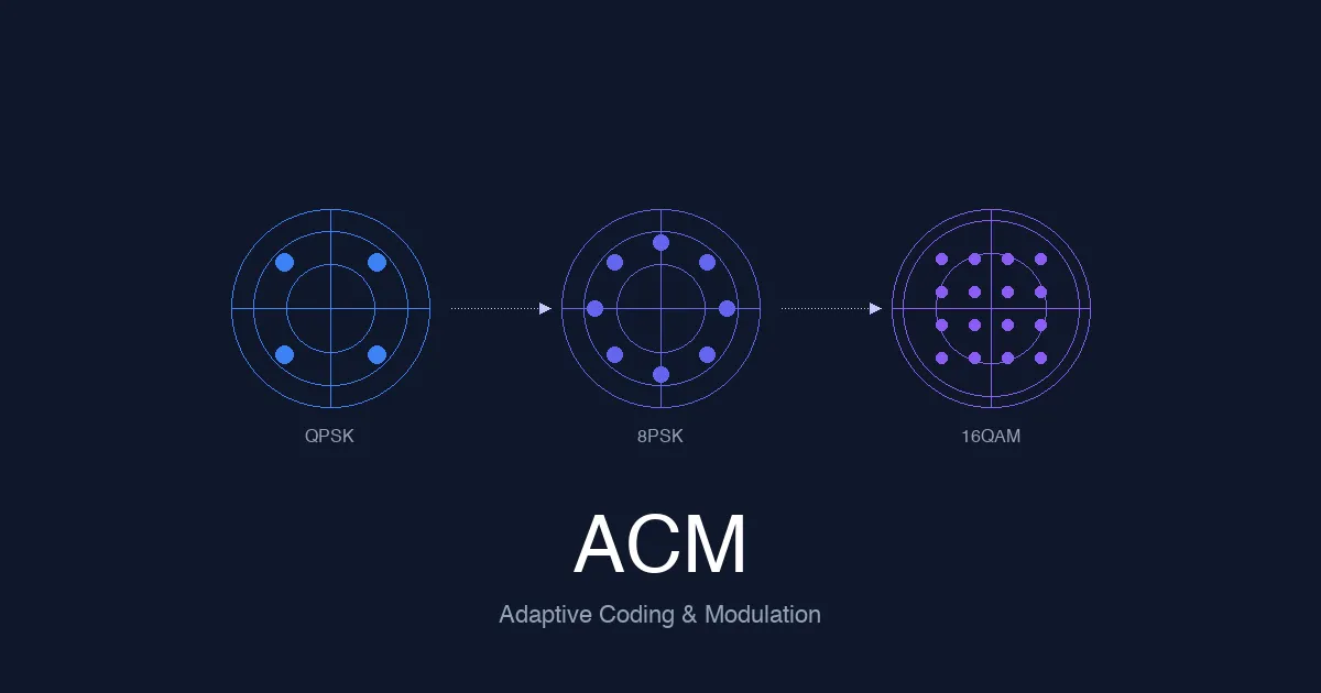
Adaptive Coding and Modulation (ACM) Explained: How Satellite Networks Maintain Link Quality
Engineering guide to adaptive coding and modulation in satellite systems covering signal quality measurement, MODCOD selection algorithms, DVB-S2/S2X ACM capabilities, rain fade response, and ACM design for HTS and LEO networks.

Satellite Glossary: M-R
Satellite communication terminology and definitions from M to R.

How Satellite Internet Works: Architecture, Latency, and Real-World Operation
Learn how satellite internet works, including GEO vs LEO satellites, ground stations, latency, and how data travels through space networks.